4 Reporting
Using papaja, it is possible to run all your analyses from within an R Markdown document.
Any output from R is included as you usually would using R Markdown.
By default the R code will not be displayed in the final documents.
If you wish to show off your code you need to set echo = TRUE in the chunk options.
This section describes how results from statistical analyses can be included into the manuscript: It starts with simple numerical values (like a sample mean) and then continues with more-complex output, like figures, tables, and the results from statistical models and hypothesis tests.
4.1 Numerical values
Consider a basic example, where you want to include a mean and a standard deviation into text:
printnum() can be used to include numeric values in the text.
The function performs the rounding and optionally omits leading zeros in accordance with APA guidelines:
Participants mean age was `r printnum(age_mean)` years ($SD = `r printnum(age_sd)`$).The above line is rendered as follows:
Participants mean age was 22.84 years (\(SD = 3.78\)).
printnum() is quiet flexible by passing its arguments to the underlying base function formatC(), so changing the number of digits after the decimal point or the character to be used to indicate the decimal point (e.g., from a point "." to a comma ",") is always possible.
papaja automatically applies printnum() to any number that is printed in inline code chunks.
Hence, `r age_mean` and `r printnum(age_mean)` are effectively identical and both yield “22.84.”
papaja additionally provides a shorthand version of printnum(), namely printp(), with defaults for correct typesetting of \(p\) values (e.g., \(p < .001\) instead of \(p = 0.000\)).
Typeset numerical values for greater control
- printnum()
- printp() as shorthand for p values
printnum(c(143234.34557, Inf))## [1] "143,234.35" "$\\infty$"printnum(42L, numerals = FALSE, capitalize = TRUE)## [1] "Forty-two"printp(c(1, 0.0008, 0))## [1] "> .999" ".001" "< .001"4.2 Figures
As in any R Markdown document, you can include figures in your document.
Figures can either consist of plots generated in R or external files.
In accordance with APA guidelines, figures are not displayed in place but are deferred to the final pages of the document.
To change this default behavior, set the option floatsintext in the YAML front matter to yes.
Figures are also saved as 300dpi PDF and PNG
- e.g.,
my_manuscript_figures/figure-latex/chunk-name-1.pdf - Change defaults using chunk options (
devanddpi)
4.2.1 R-generated figures
Any plot that is generated by an R code chunk is automatically included in your document.
Hence, a simple call to plot() is sufficient to create a figure:
plot(cars)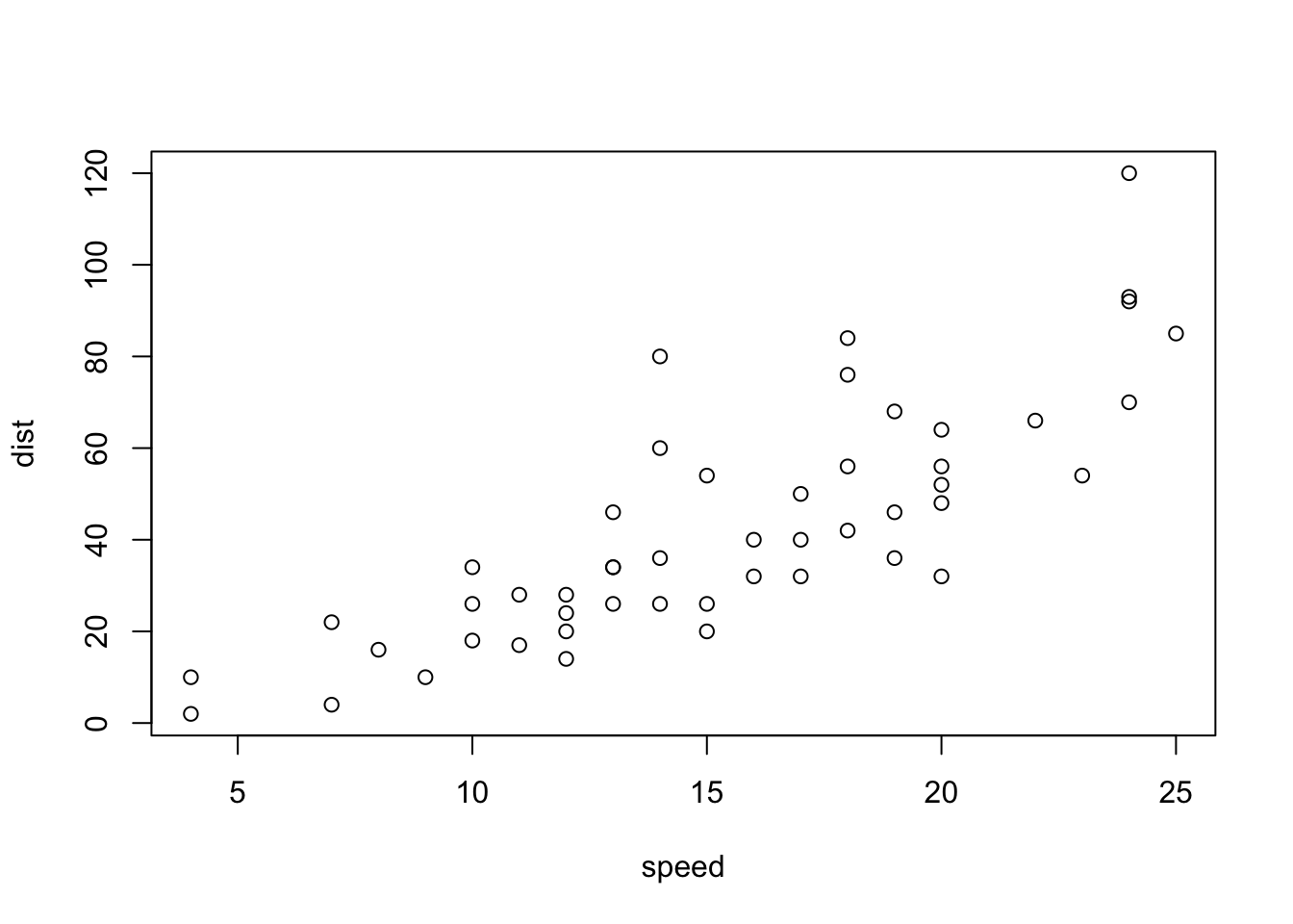
Figure 4.1: A basic scatterplot of the cars dataset.
Figure display size, resolution, file format and many other things can be controlled by setting the corresponding chunk options.
Refer to the plot-related knitr chunk options for an overview of all options.
In papaja-documents, by default, all figures are saved as vectorized PDF and pixel-based PNG files at a resolution of 300 DPI, which should in most cases be sufficient for a print publication.
When the target document format is PDF the vectorized PDF files are included; when the target document format is DOCX the pixel-based PNG files are included.
The files can be found in the mydocument_files folder that is generated when mydocument.Rmd is knitted.
Note, if you define transparent colors in your plots (e.g., when you define colors using rgb()), the rendered document will always display the pixel-based PNG files, regardless of the target document format.
Given the lossless compression in PNG and the decent resolution of 300 DPI this should not be a problem in print.
4.2.1.1 papaja plot functions
Factorial designs are ubiquitous in experimental psychology, but notoriously cumbersome to visualize with R base graphics.
That is why papaja provides a set of functions to facilitate plotting data from factorial designs.
The functions apa_beeplot(), apa_lineplot(), apa_barplot(), and the generic apa_factorial_plot() are intended to provide a convenient way to obtain a publication-ready figure while maintaining enough flexibility for customization.
The basic arguments to these functions are all the same, so you only need to learn one syntax to generate different types of plots.
Moreover, it is easy to switch between the different types of plots by only changing a few letters of the function name.
Consider the following example of a so-called beeswarm plot:
apa_beeplot(
  data = mixed_data
  , id = "Subject"
  , dv = "Recall"
  , factors = c("Task", "Valence", "Dosage")
)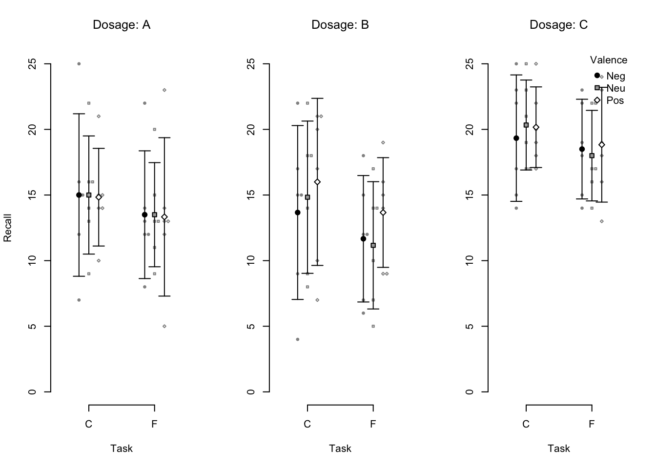
Figure 4.2: An example beeswarm plot. Small points represent individual observations, large points represent condition means, and error bars represent 95% confidence intervals.
A data.frame that contains the data in long format is passed to the data argument.
The other arguments expect the names of the columns that contain the subject identifier id,
the dependent variable dv, and the between- or within-subjects factors of the design.
Currently, zero to four factors are supported.
For each cell of the design, the functions plot
- central tendency,
- dispersion, and
- names of dependent variable, factors and levels, and optionally a legend.
Mesures of central tendency and dispersion default to the mean and 95% confidence intervals.
However, the arguments tendency and dispersion can be used to overwrite these defaults and plot other statistics.
For example, to plot within-subjects rather than between-subjects confidence intervals you can set dispersion = within_subjects_conf_int.
If the data encompass multiple observations per participant-factor-level-combination, these observations are aggregated.
By default, the condition means are computed but you can specify other aggregation functions via the fun_aggregate argument.
The visual elements of the plots can be customized by passing options to the arguments args_points, args_error_bars, args_legend, and so on.
These arguments take named lists of arguments that are passed on to the respective functions from the graphics package (which comprises R’s standard plotting functions), such as points(), arrows(), and legend().
Consider the following code and the resulting Figure 4.3 for a customized version of the previous beeswarm plot.
apa_beeplot(
    data = mixed_data
  , id = "Subject"
  , dv = "Recall"
  , factors = c("Task", "Valence", "Dosage")
  , dispersion = within_subjects_conf_int
  , main = c(expression(italic(A)~"dosage"), expression(italic(B)~"dosage"), expression(italic(C)~"dosage"))
  , ylab = "Number of correctly recalled words"
  , args_points = list(cex = 2, bg = c("skyblue4", "indianred3", "seagreen4"), col = "white")
  , args_swarm = list(cex = 1.2)
  , args_error_bars = list(length = 0.02, col = "grey20")
  , args_legend = list(x = "bottom", inset = 0.05)
  , args_y_axis = list(las = 1)
)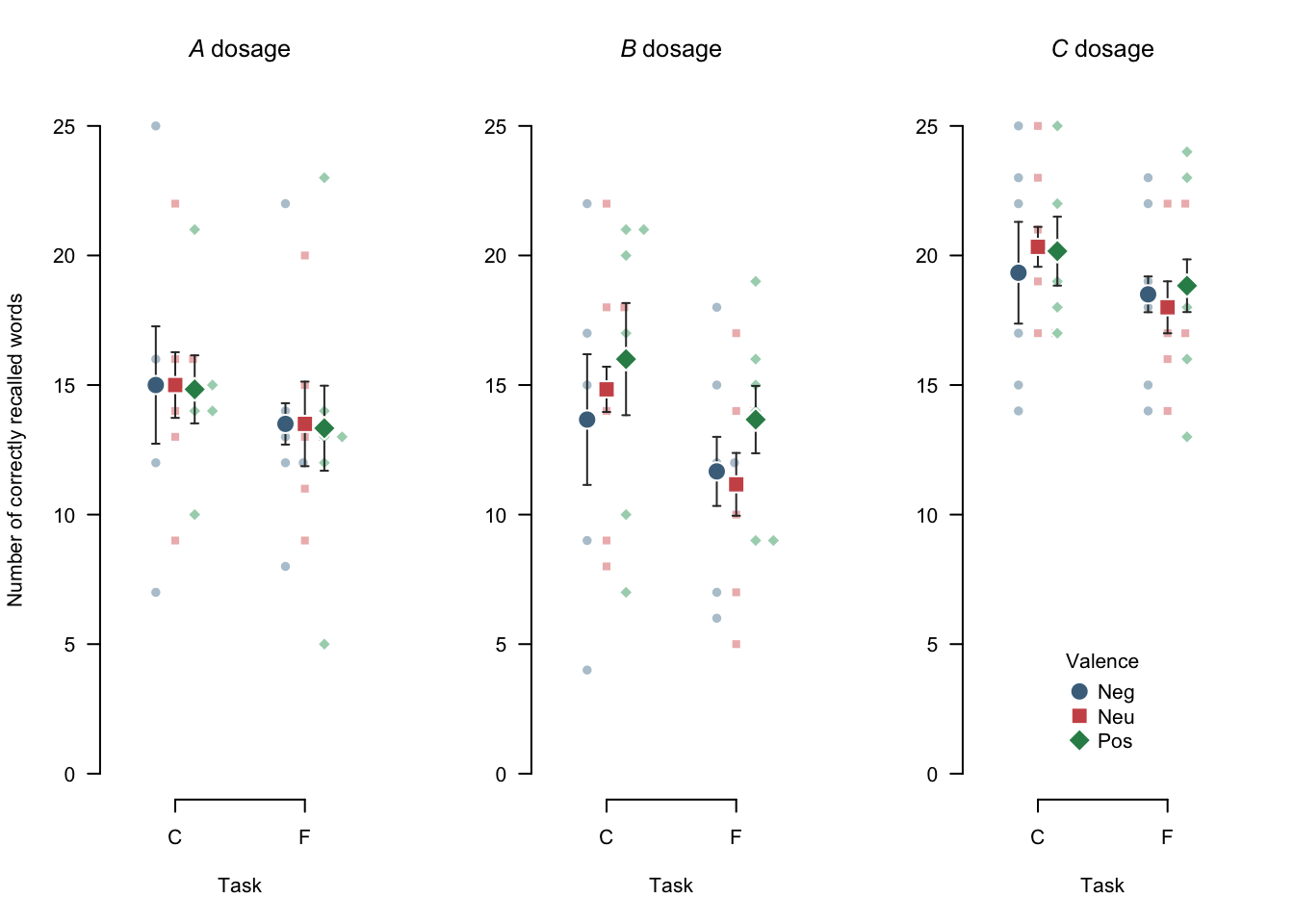
Figure 4.3: A customized beeswarm plot. Note that, by default, the swarm inherits parameters from the args_points argument. Small points represent individual observations, large points represent means, and error bars represent 95% within-subjects confidence intervals.
- Utilize variable labels
These plot functions also utilize variable labels, with some \(\LaTeX\) math support (see ?latex2exp::TeX)
variable_labels(cosmetic_surgery) <- c(
  Post_QoL = "Quality of life post surgery ($\\bar{x}_{post}$)"
)

apa_beeplot(
  id = "ID"
  , dv = "Post_QoL"
  , factors = c("Reason", "Surgery", "Gender")
  , data = cosmetic_surgery
  # , ylab = "Quality of life post surgery"
  , las = 1
  , args_legend = list(x = 0.25, y = 30)
  , args_points = list(bg = c("skyblue2", "indianred1"))
  , args_error_bars = list(length = 0.03)
)
4.2.1.2 Setting global plot options
As noted in the APA guidelines (p. 153) figures in an article should be consistent and in the same style.
Hence, it is desirable to define plot styles only once, rather than every time a new plot is created.
When using graphics plot functions global options can be set using par().
For example, the size of labels and symbols can be controled with cex:
par(cex = 1.2)
apa_beeplot(
  data = mixed_data
  , id = "Subject"
  , dv = "Recall"
  , factors = c("Task", "Valence")
)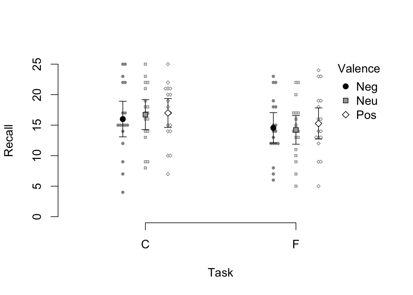
Figure 4.4: A variant of the example beeswarm plot with larger labels and symbols.
However, the use of par() is restricted in knitr.
knitr resets par() for every chunk; par() needs to be called anew in every chunk that creates a plot.
While there are advantages to this behavior it impedes defining a consistent plot style.
Although not very convenient, it is possible to set global plot options in knitr and therefore also in papaja.
The following example illustrates how to make knitr execute a specified call to par() before executing code in a given chunk.
Here we rotate the \(y\)-axis label (las = 1), set a regular font and increase the size of the main title (font.main = 1, cex.main = 1.05).
# Ensure that par()-settings are retained across chunks
knitr::opts_knit$set(global.par = TRUE)
# Define a function that sets desired global plot defaults
par(font.main = 1`, `cex.main = 1.05, las = 1)The customizations apply to all subsequently generated plots. It is, thus, advisable to add this code at the top of the R Markdown document shortly after the YAML front matter.
The aforementioned limitations do not apply to users of ggplot2.
Custom themes can be set as default as usual and are subsequently applied to all plots created with ggplot().
papaja provides a template theme_apa() that we feel is well suited to create publication-ready plots.
The following example demonstrates how to set a default theme.
# Cosmetic surgery dataset from
# Field, A. P., Miles, J., & Field, Z. (2012). Discovering statistics using R. London: Sage.
load("data/cosmetic_surgery.rdata")

ggplot(
    cosmetic_surgery
    , aes(x = Base_QoL, y = Post_QoL, color = Reason)
  ) +
  geom_point() +
  geom_smooth(method = "lm") +
  labs(
    x = "Baseline quality of life"
    , y = "Quality of life post surgery"
  ) +
  scale_color_brewer(palette = "Set1") +
  theme_apa(box = TRUE) +
  theme(legend.position = c(0.2, 0.8))
## `geom_smooth()` using formula 'y ~ x'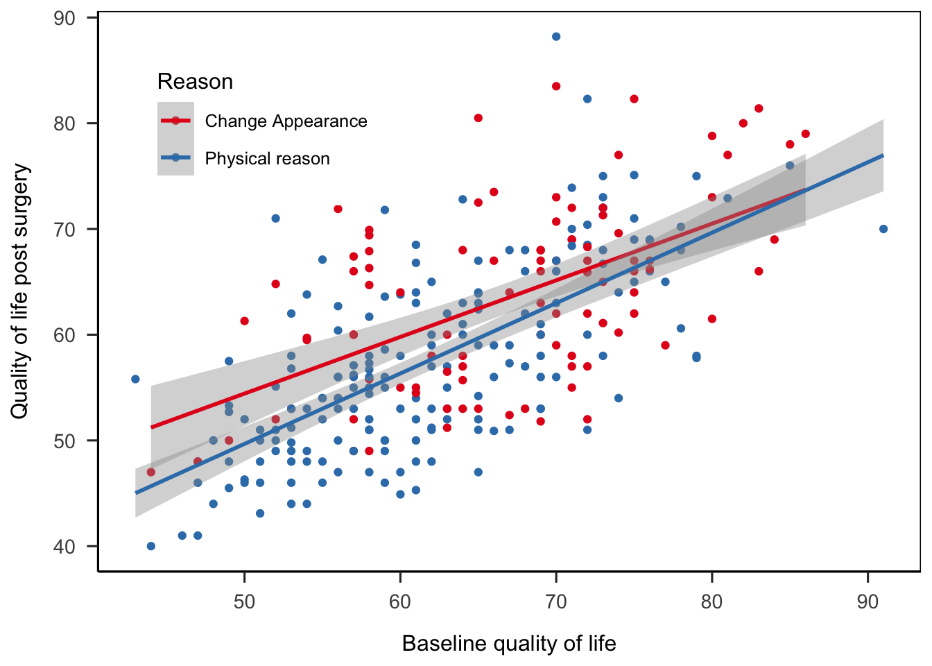
theme_set(theme_apa())4.2.2 External images
External images are best included by using knitr::include_graphics(), e.g.
knitr::include_graphics("images/swans.png")
Figure 4.5: Only from observing many white swans, you cannot conclude that all swans are white.
4.2.3 Figure captions
The chunk option fig.cap sets a figure caption.
You can define a figure caption simply by passing a character string to fig.cap:
```{r my-figure, fig.cap = "My caption."}
plot(cars)
```
However, we strongly recommend that you use Text references instead:
(ref:my-figure-caption) My caption.

```{r my-figure, fig.cap = "(ref:my-figure-caption)"}
plot(cars)
```
It’s best to define the text reference for a caption just above the corresponding code chunk. For details see Text references.
fig.cap is used for all figures that are created in the respective chunk.
If multiple figures are created the caption will be duplicated.
Unless this behavior is desired, only one figure should be created per chunk.
Alternatively, you can combine multiple plots into one figure, for example using layout(), cowplot, or patchwork.
Note that long figure captions may flow over the page of a PDF document. There are two approaches to accomodate long figure captions or tall figures. You can adjust the line spacing/font size of the caption or use a separate list of figure captions. As mentioned Adjusting line spacing, you can adjust the line spacing and font size of figure captions. For single-spaced script-size figure captions, add the following to the YAML front matter:
header-includes:
  - \usepackage{setspace}
  - \captionsetup[figure]{font={stretch=1,scriptsize}}
For other font size options see the LaTeX Wikibook.
To add a list of figure captions after the reference section, add the following to the YAML front matter:
figurelist: yesIf you additionally want to suppress the captions below all figures, you can add the following LaTeX code to the document preamble:
header-includes:
  - \captionsetup[figure]{textformat=empty}
If you would rather suppress figure captions only where they do not fit the page, you can instead make knitr do this.
To remove the caption below a figure set fig.cap = " " and instead set the figure short caption via the chunk option fig.scap = "My figure caption":
    (ref:figure-caption) This is a long figure caption!

    ```{r fig.cap = " ", fig.scap = "(ref:my-figure-caption)", out.width = "\\textwidth"}
    plot(cars)
```fig.scap takes effect, knitr requires that the chunk specifies out.width, out.height, or fig.align, as explained here.
4.3 Tables
There are many available functions and packages to create tables in R Markdown documents.
As a default option knitr::kable() is a good choice.
papaja also provides a funtion to create tables—apa_table().
apa_table() is an extension of knitr::kable(), so all the options you know from kable() will work with apa_table().
library(dplyr)
descriptives <- mixed_data %>% group_by(Dosage) %>%
  summarize(
    Mean = mean(Recall)
    , Median = median(Recall)
    , SD = sd(Recall)
    , Min = min(Recall)
    , Max = max(Recall)
  )
descriptives[, -1] <- printnum(descriptives[, -1])

apa_table(
  descriptives
  , caption = "Descriptive statistics of correct recall by dosage."
  , note = "This table was created with apa_table()."
  , escape = TRUE
)| Dosage | Mean | Median | SD | Min | Max |
|---|---|---|---|---|---|
| A | 14.19 | 14.00 | 4.45 | 5 | 25 |
| B | 13.50 | 14.00 | 5.15 | 4 | 22 |
| C | 19.19 | 19.00 | 3.52 | 13 | 25 |
Note. This table was created with apa_table().
apa_table() creates tables that are inspired by the examples presented in the APA manual and that adhere to its guidelines.
Unfortunately, in papaja table formatting is somewhat limited for Word documents due to missing functionality in pandoc (e.g., it is not possible to have cells or headers span across multiple columns).
The function performs no calculations but simply prints any data.frame it is given.
If you pass a list to apa_table(), all list elements are merged by columns into a single data.frame and the names of list elements are added to the table according to the setting of merge_method.
When using apa_table(), the type of the output (LaTeX or MS Word) is determined automatically by the rendered document type.
In interactive R session (unless a document is being rendered) the output defaults to LaTeX.
To use LaTeX code inside a table you have to set escape = FALSE.
Otherwise, elements of the LaTeX syntax (such as backslashes) will be printed as is.
If you set escape = FALSE you need to manually escape symbols that would otherwise be interpreted as LaTeX code, such as underscores (see note in the example below).
When you pass backslashes as character strings you need to escape the backslash with one additional backslash because R uses backslashes to denote special characters, such as \t for tab or \n for newline.
If you would like to add mathematical symbols in any part of the table use $ (not $$, which is used in-text) to denote the beginning and end of the mathematical expression.
As required by the APA guidelines, tables are deferred to the final pages of the manuscript when creating a PDF.
To place tables and figures in your text instead, set the figsintext parameter in the YAML header to yes or true, as I have done in this document.
Again, this is not the case in Word documents due to limited pandoc functionality.
The bottom line is, Word documents will be less polished than PDF.
The resulting documents should suffice to enable collaboration with Wordy colleagues and prepare a journal submission with limited manual labor.
4.3.1 Fixed-width columns
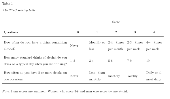
By default, the width of the table is set to accommodate its contents. In some cases, this may cause the table to exceed the page width. To address this, in PDF documents tables can be rotated 90 degrees by setting . This approach, however, is not particularly useful if one of the columns contains long texts, such as survey question texts. In such cases, it is possible to create fixed-width columns by explicitly specifying the desired column widths. Such fixed-width colums automatically break the content into multiple lines. For example, set to limit the second column to a width of 5 cm. Consider the following example of a table summarizing the scoring rules of the AUDIT-C scale (Bradley et al., 2007), curtosey of James Conigrave.
audit_table <- structure(
  list(
    Questions = c(
      "How often do you have a drink containing alcohol?",
      "How many standard drinks of alcohol do you drink on a typical day when you are drinking?",
      "How often do you have 5 or more drinks on one occasion?"
    ),
    `0` = c("Never", "1–2", "Never"),
    `1` = c("Monthly or less", "3-4", "Less than monthly"),
    `2` = c("2-4 times per month", "5-6", "monthly"),
    `3` = c("2-3 times per week","7-9", "Weekly"),
    `4` = c("4+ times per week", "10+", "Daily or almost daily")
  ),
  class = "data.frame",
  row.names = c(NA, 3L)
)

apa_table(
  audit_table,
  caption = "AUDIT-C scoring table",
  align = c("m{8cm}", rep("m{2cm}", 5)),
  col_spanners = list("Score" = c(2,6)),
  note = "Item scores are summed. Women who score 3+ and men who score 4+ are at-risk",
  landscape = TRUE
)
Similarly, to space columns equally use align = paste0("m{", 1/(ncol(x) + 1), "\\linewidth}").
4.3.2 Table captions
As shown above, table captions can be created by passing a character string to caption = argument within apa_table function (e.g. apa_table(descriptives, caption = "My table caption.")).
However, we strongly recommend that you use Text references instead:
(ref:my-table-caption) My caption.

```{r my-table}
apa_table(descriptives, caption = "(ref:my-table-caption)")
```
It’s best to define the text reference for a caption just above the corresponding code chunk. For details see Text references.
4.3.3 Alternatives
Pixidust: https://github.com/nutterb/pixiedust/blob/master/README.md
xtable: https://cran.r-project.org/web/packages/xtable/xtable.pdf
tables: https://cran.r-project.org/web/packages/tables/vignettes/tables.pdf
stargazer: https://cran.r-project.org/web/packages/stargazer/index.html
Hmisc::latex
https://twitter.com/polesasunder/status/464132152347475968/photo/1
kableExtra: https://cran.r-project.org/web/packages/kableExtra/index.html
4.4 Statistical Models and Tests
When creating reproducible reports of quantitative results, it will be necessary to include the results from statistical models and tests. However, what comes out of R cannot be included in a report easily. Consider the output from a simple t test:
t.test(yield ~ N, data = npk)##
## Welch Two Sample t-test
##
## data: yield by N
## t = -2.4618, df = 21.88, p-value = 0.02218
## alternative hypothesis: true difference in means is not equal to 0
## 95 percent confidence interval:
## -10.3496778 -0.8836555
## sample estimates:
## mean in group 0 mean in group 1
## 52.06667 57.68333We created the function apa_print() to format the results from various statistical methods in accordance with APA guidelines.
Just drop the results from these methods into apa_print(), and it will return a simple list with all you need to report the analysis.
apa_print(
  t.test(yield ~ N, data = npk)
)
## $estimate
## [1] "$\\Delta M = -5.62$, 95\\% CI $[-10.35, -0.88]$"
##
## $statistic
## [1] "$t(21.88) = -2.46$, $p = .022$"
##
## $full_result
## [1] "$\\Delta M = -5.62$, 95\\% CI $[-10.35, -0.88]$, $t(21.88) = -2.46$, $p = .022$"
##
## $table
## A data.frame with 5 labelled columns:
##
## estimate conf.int statistic df p.value
## 1 -5.62 [-10.35, -0.88] -2.46 21.88 .022
##
## estimate : $\\Delta M$
## conf.int : 95\\% CI
## statistic: $t$
## df : $\\mathit{df}$
## p.value : $p$
## attr(,"class")
## [1] "apa_results" "list"The returned list contains four elements:
$estimate: A character string that holds the information about original-scale and/or standardized estimates of the model term.$statistic: A character string that holds the result of the NHST with test statistic, dfs, and p value;$full_result: combines this information.$table: arranges model terms, estimates and test statistics in adata.frame
List elements $estimate, $statistic, and $full_result are intended to be included directly into the body of your manuscript by using inline code chunks.
For instance, you could first save the result from apa_print() in an output object
out <- apa_print(
  t.test(yield ~ N, data = npk)
)
and then include a single list element by writing:
Plant yield indeed differed between groups, `r out$full_result`.The above line is rendered as follows:
Plant yield indeed differed between groups, \(\Delta M = -5.62\), 95% CI \([-10.35, -0.88]\), \(t(21.88) = -2.46\), \(p = .022\).
The last element $table is intended to be used to create results tables that may be included in the manuscript via apa_table().
It will be most useful for analyses that contain multiple hypothesis tests, as you will see in the next subsections.
4.4.1 Reporting models and tests in a table
For statistical models with multiple terms (for instance, multiple regression or multi-way ANOVA) it is sometimes convenient
to report the statistical tests of all model terms in a table.
For this purpose, apa_print() returns the list element $table that may be included using function apa_table() or any other table
(for instance, kable() from the {knitr} package).
Consider the following regression model
lm_out <- lm(formula = Post_QoL ~ Base_QoL + BDI, data = cosmetic_surgery)
summary(lm_out)
##
## Call:
## lm(formula = Post_QoL ~ Base_QoL + BDI, data = cosmetic_surgery)
##
## Residuals:
## Min 1Q Median 3Q Max
## -14.2178 -4.9922 -0.2825 4.1874 24.1555
##
## Coefficients:
## Estimate Std. Error t value Pr(>|t|)
## (Intercept) 18.50378 2.74711 6.736 9.63e-11 ***
## Base_QoL 0.58625 0.04430 13.233 < 2e-16 ***
## BDI 0.16680 0.02743 6.082 4.00e-09 ***
## ---
## Signif. codes: 0 '***' 0.001 '**' 0.01 '*' 0.05 '.' 0.1 ' ' 1
##
## Residual standard error: 6.596 on 273 degrees of freedom
## Multiple R-squared: 0.5005, Adjusted R-squared: 0.4969
## F-statistic: 136.8 on 2 and 273 DF, p-value: < 2.2e-16To include the model table into your manuscript, first apply apa_print() to the model object,
and then use apa_table() on the list element $table.
apa_lm <- apa_print(lm_out)
apa_table(
  apa_lm$table
  , caption = "A full regression table."
)| Predictor | \(b\) | 95% CI | \(t(273)\) | \(p\) |
|---|---|---|---|---|
| Intercept | 18.50 | [13.10, 23.91] | 6.74 | < .001 |
| Base QoL | 0.59 | [0.50, 0.67] | 13.23 | < .001 |
| BDI | 0.17 | [0.11, 0.22] | 6.08 | < .001 |
4.4.2 Supported analysis methods
There is a plethora of possible output objects from statistical analyses in R, and it is of course impossible to support all of them. However, over the course of time, we were able to create a corpus of methods that will likely cover many experimental psychologists’ toolboxes.
- All NHST that are delivered with R’s {stats} package, which includes:
- \(t\) for means, \(\chi^2\), and nonparametric equivalents
t.test() - tests for correlation coefficients
cor.test() - (generalized) linear models
- …
- except for pairwise comparisons (these should be done with the package {emmeans})
- \(t\) for means, \(\chi^2\), and nonparametric equivalents
- Analysis of Variance ANOVA and ANCOVA (from packages {stats}, {car}, and {afex})
- Multivariate Analysis of Variance MANOVA and MANCOVA (from {stats})
- Hierachical (Generalized) Linear Models (from {lme4}, {lmerTest}, {nlme}, and {afex})
- Pairwise comparisons and planned contrasts from {emmeans}, {lsmeans}, and {glht} (these methods are still experimental)
- Bayesian t tests and ANOVAs from {BayesFactor}
There are gaps that we would like to fill, see section 10.
| A-B | B-L | L-S | S-Z |
|---|---|---|---|
| afex_aov | BFBayesFactorTop* | lme | summary.aov |
| anova | default | lsmobj* | summary.aovlist |
| anova.lme | emmGrid* | manova | summary.glht* |
| Anova.mlm | glht* | merMod | summary.glm |
| aov | glm | mixed | summary.lm |
| aovlist | htest | papaja_wsci | summary.manova |
| BFBayesFactor* | list | summary_emm* | summary.ref.grid* |
| BFBayesFactorList* | lm | summary.Anova.mlm |
* Not fully tested, don’t trust blindly!
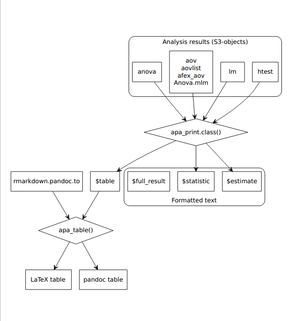
Figure 4.6: Process diagram illustrating the use of apa_print() methods and apa_table() to format results from statistical analyses according to APA guidelines. The formatted text and tables can be reported in a manuscript.
4.4.2.1 Model Comparisons for Linear (Mixed-Effects) Models
…
4.4.2.2 Analysis of Variance ANOVA
You can skip this if you are not interested in technical background.
Amongst psychologists, analysis of variance is a still-popular and frequently used technique.
In base R, however, analysis of variance is not implemented in a way that is too useful
for psychologists, as the aov-function in the stats package does not provide the much sought-after
Type-\(\rm{I\!I\!I}\) sums-of-squares. A variety of R packages has emerged to fill the gap, e.g.
{car} (Fox & Weisberg, 2011), {ez} (Lawrence, 2016), and {afex} (Singmann, Bolker, Westfall, & Aust, 2016).
Unfortunately, each ANOVA function provides different output objects that need to be digested by apa_print().
To do so, we rely on the package authors to return standardized result objects (i.e., S3/S4 classes).
For this reason apa_print() does not support results from the popular ezANOVA().
The object returned by this function has no class to inform us about its contents and, thus, cannot be processed.
We recommend you try one of the other available packages, e.g. aov_ez() from the afex-package.
Functionality.
cosmetic_surgery_anova <- afex::aov_ez(
  data = cosmetic_surgery
  , dv = "Post_QoL"
  , id = "ID"
  , between = c("Clinic", "Gender")
)
apa_anova <- apa_print(cosmetic_surgery_anova)
Now, you can report the results of your analyses like so:
Clinic (`r apa_anova$full$Clinic`) and patient gender affected post-surgery quality of life, `r apa_anova$full$Gender`. However, the effect of gender differed by clinic, `r apa_anova$full$Clinic_Gender`.Which will yield the following text:
Clinic (\(F(9, 256) = 19.98\), \(\mathit{MSE} = 47.58\), \(p < .001\), \(\hat{\eta}^2_G = .413\)) and patient gender affected post-surgery quality of life, \(F(1, 256) = 15.29\), \(\mathit{MSE} = 47.58\), \(p < .001\), \(\hat{\eta}^2_G = .056\). However, the effect of gender differed by clinic, \(F(9, 256) = 1.97\), \(\mathit{MSE} = 47.58\), \(p = .043\), \(\hat{\eta}^2_G = .065\).
Again, you can easily create a complete ANOVA table by passing $table to apa_table(), see .
apa_table(
  apa_anova$table
  , caption = "A really beautiful ANOVA table."
  , note = "Note that the column names contain beautiful mathematical copy: This is because the table has variable labels."
)| Effect | \(\hat{\eta}^2_G\) | \(F\) | \(\mathit{df}\) | \(\mathit{df}_{\mathrm{res}}\) | \(\mathit{MSE}\) | \(p\) |
|---|---|---|---|---|---|---|
| Clinic | .413 | 19.98 | 9 | 256 | 47.58 | < .001 |
| Gender | .056 | 15.29 | 1 | 256 | 47.58 | < .001 |
| Clinic \(\times\) Gender | .065 | 1.97 | 9 | 256 | 47.58 | .043 |
Note. Note that the column names contain beautiful mathematical copy: This is because the table has variable labels.
4.4.2.3 Post-hoc Comparisons and Planned Contrasts
We are currently working on full support of post-hoc tests, contrasts and expected
marginal means from the emmeans and lsmeans packages. A lot of work has already
been done and you may use the available methods, but you should double-check
the results because these new methods are not fully tested, yet.
The same applies to results returned by the glht() function from package multcomp.
4.4.2.4 Mixed-effects Models
We are currently working on full supoort of mixed effects
4.5 Caching expensive computations
If R codes take a long time to run, results can be cached
```{r heavy-computation, .highlight[cache = TRUE]}
# Imagine computationally expensive R code here

```
my_manuscript_cache directory is created that contains
- Computed objects
- List of loaded R packages in __packages
The next time the chunk is executed
- If unchanged, cached results are loaded
- If changed, cache is discarded and code is executed anew
Packages are not reloaded, which causes problems in subsequent uncached chunks
- Do not include
library()-calls in cached chunks!
Load cache into an interactive R session using lazyLoad()
library()-calls.
Subsequent use of functions from these packages in non-cached chunks will throw errors!
To avoid incorrect results due to caching, dependencies should be specified
```{r chunk1, cache = TRUE}
x <- 5

```
```{r chunk2, cache = TRUE, .highlight[dependson = “chunk1”]}
x <- x + 5

```
If code in chunk1 changes, chunk2 is recomputed
To avoid incorrect results due to caching, dependencies should be specified
knitr::opts_chunk$set(autodep = TRUE)
knitr::dep_auto()
See knitr cache examples for details
Control when cache is discarded
- Ignore changes to comments
knitr::opts_chunk$set(cache.comments = FALSE)- Discard cache when random seed changes
opts_chunk$set(cache.extra = knitr::rand_seed)I would recommend to always set these options
- Discard cache if data are modified
opts_chunk$set(cache.extra = file.info("data.csv")$mtime)- Discard cache if the R environment changes
opts_chunk$set(
  cache.extra = list(R.version, sessionInfo())
)
If time permits, always discard all cached results (i.e., delete my_manuscript_cache directory) and reknit the document before submission to ensure that all results are based on the current R code!
4.5.1 Inserting variables before they have been computed
R code in R Markdown documents in executed from top to bottom. Hence, variables are not available before the code chunk in which they are defined has been executed. However, sometimes it may be desireable to report a variable in a document before the corresponding code chunk. A common example is to include the sample size or focal test statistics in the abstract.
Cached code chunks store their results in a cache database in the subfolder my_document_cache (default).
The function knitr::load_cache() can be used to access cache databases and report results of a chunk anywhere in the document.
For the following example, we’ll assume that we want to report the sample size in the abstract.
The sample size is calculated in the method section:
```{r, sample-size, cache = TRUE}
n <- nrow(cosmetic_surgery)
```
To report this variable in the abstract we need to use an inline code chunk in the YAML front matter field:
---
abstract: |
  This is the abstract.
  Our sample size was n = `r knitr::load_cache(label = "sample-size", object = "n")`.
---
When the document is first rendered the object n in the code chunk sample-size has not yet been computed and knitr::load_cache() will insert "NOT AVAILABLE" instead.
The next time the document is rendered, the results of the previous run have been saved as cache database.
These results will be loaded and inserted into the abstract.
knitr::load_cache() can only ever display the result of the previous run—if the cached code is changed, the document has to be rendered twice to display the new result.